Please accept my apologies for the poor recent support for Understanding the Properties of Matter.
The basic issue arose because the software that I used to create the site (Adobe Go Live) became obolete making editing a tedious manual job using bare HTM. Then the long-standing web host for the site went out of business and I was unable to move the site to a new web-hosting service. This was because of a tragic combination of busy-ness and technical incompetence. And with one thing and another, I have been very tardy at moving resources from my back up files to this new WordPress hosted blog.
But here we are and I have decided to take the opportunity to make a few changes.
Free!
From now on, the pdfs of each chapter will be available for free unrestricted download. Why?
As I explained on the previous, now lost, website, writing academic texts is not a money-making activity. I wrote the book because I loved this subject. And I still do.
It might seem that in order to make the book last beyond a few years one might rely on publishers to promote the text and perhaps provide some kind of ongoing support. Unfortunately there has been absolutely no support from the publishers – I am sure they have more important things to do than sell this type of book. Additionally the text book has become very expensive. So in order to make the book sustainable I think the best option is to simply release it. Some students are not well off and free is a great price!
Support
I am now a retired person and although I am happily very busy, I hope to have some time to improve the support for the book. In particular I hope to:
Reconstruct the functionality from the previous web site in terms of downloads of tables, and figures.
Revise the figures to use colour where relevant and incorporate them into PowerPoint slides.
Revise the answers to the questions and the extended questions.
Publish the tables of errata that I have been sent!
Plus whatever else occurs to me – or that you ask me to do!
I intend to have a blitz on this during this the last week of March 2021. There are a thousand technical difficulties with every single step on that list of bullet points, from file incompatibility errors to appalling editors. But these details don’t matter. My aim is to have the site presentable again by the end of March 202: do let me know if there is anything you want to see.
I received a delightfully-worded request for clarification from a correspondent in India the other day. I say “delightfully-worded” because the correspondent started out by complimenting me :-).
The enquiry concerned a subtle detail of the band theory of solids that requires an understanding of the way the band gap affects electronic states in two or three dimensions.
This extension beyond one dimension is particularly difficult to visualise.
Anyway: here is the letter: my response is below.
Dear Michael,
I have read the web chapter on the band theory of solids in physicsofmatter. I really enjoyed reading for its clarity of expression.
It was most elegantly presented than elsewhere on web or books. Thank you for creating such a wonderful document.
But, I could not follow the following paragraph:
Figure W1.15 shows how the energy varies as one proceeds from the origin along lines joining the origin to the point (0, ¹/a) and to the point ( ¹/a, ¹/a). Notice that the magnitude of the parameter Vo in Equation 1.80 now becomes very important.
If Vo is large compared with the maximum energy of a quantum state in the first Brillioun zone, then all the quantum states in the second Brillioun Zone will have energies higher than any quantum state in the first Brillioun Zone. In this situation there is what is known as a band gap between states in the two zones. ·
However, if Vo is small compared with the maximum energy of a quantum state in the first Brillioun zone, then some of the quantum states in the second Brillioun Zone will have energies lower than some quantum states in the first Brillioun Zone. In this situation there is said to be band overlap between states in the two zones.
The point I did not understand is precisely this “second Brillioun Zone will have energies lower than some quantum states in the first Brillioun Zone. In this situation there is said to be band overlap between states in the two zones.” I do not see any band overlap in the figure or see any quantum states in second zone whose energy is lower than the first zone. I know, I am missing something but can not figure out what it is? Can you please help me in understanding this point?
The letter refers to Figure W1.15 which looks like this:
Figure W1.15 Illustration of the results of two-dimensional, nearly-free electron calculation for the case of two electrons per lattice site. (a) (b) and (c) correspond to the case when V0 is large and (d) (e) and (f) to the case when V0 is small. (a) and (d) show the structure of E(k) along k,0,0 and k,k,0 directions (b) and (e) show the resulting density of states. Notice that in (b) the density of states at the Fermi energy is zero which is indicative of insulator. (c) and (f) show three dimensional views of the band structure in the two bands
The key point can be seen if we enlarge part (f) of the above figure:
Part (f) of the figure above with key points highlighted.
The key point is that if the splitting between the upper and lower band is small, then the lowest point in the upper band (yellow square) is lower in energy than the highest point in the lower band (yellow circle).
The perspective of the drawing means that I can’t clearly show all the symmetrically equivalent points in this diagram. So I have shown only one of the four equivalent points in the upper band (square), and three of the four equivalent points in the lower band (circles)
Because of this, a material with such a band structure would have electronic states (occupied or unoccupied) at every energy, so there would be no energy gap. This is illustrated in part (e) of Figure W1.15.
This contrasts with the case shown in part (c) of Figure W1.15
Part (c)
Now we can see that if the splitting between the upper and lower band is large, then the lowest points in the upper band (yellow square) are higher in energy than even the highest point in the lower band (yellow circles).
Because of this, in a material with such a band structure would there would be an energy gap where there were no states that could be occupied by electrons. This is illustrated in part (b) of Figure W1.15.
A reminder of why this matters.
The reason that this kind of analysis matters is that it allows us to explain astonishing qualitative differences between materials in terms of a single quantitative parameter – in this case Vo.
So for example argon and potassium are spectacularly different materials. We know from §6.2 and §7.3, that argon is a gas at room temperature and forms a ‘molecular solid’ at low temperatures.
However, when we describe potassium, we would naturally discount the theory for argon as irrelevant, and use the theory for a free electron gas described in §6.5.
But argon and potassium atoms differ by only a single electron in their outer electronic shells. Can we find a theory that explains why the addition of a single electron per atom makes potassium a metal? This is what the band theory of solids does.
The band theory of solids is essentially a framework that allows us to discuss the nature of electronic states in all kinds of solids, and to explain from first principles why one type of atom forms solids that are insulating, and other similar atoms form solids that are metals.
The two most important of the ‘neglected details’ in the theory of a gas turn out to be the finite size of the molecules and their mutual interactions. Johannes Diderik van der Waals understood this and developed a modified version of the ideal gas equation PV = nRT
In this equation there are two new parameters a and b which characterise the effect of the neglected details.
The parameter a characterises the way in which the electrical attraction between molecules – also described by Van der Waals – reduces the pressure below that which would be expected for an ideal gas. The squared-dependence on molar density, ρ, arises from two effects.
Firstly in this simple model,the number of attractive interactions a single molecule experiences depends on the number of molecules in its vicinity and so is proportional to ρ
Secondly, the effect on the pressure depends on the number of molecules per unit volume and so is proportional to ρ
Combining these two effects leads to an effect proportional to ρ2.
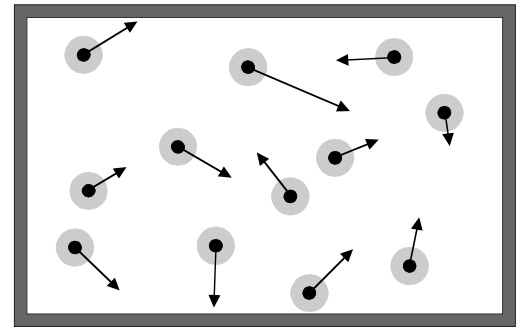
The parameter b characterises the finite volume occupied by the molecules themselves. We would expect this to be roughly equal to the molar volume of the substance when in it is in a solid or liquid state.
There’s a table of values of a and b parameters for a range of gases at the end of this article, but before we get calculating, it is worth noting that there are several really interesting things about this equation.
Interesting thing#1. As I mentioned in the previous article, the deviations from the ideal gas equation arise from the basic interactions between molecules. And so if we can measure these deviations from the ideal gas equation we can deduce the properties of molecular interactions. That’s right: precision measurements of mundane macroscopic properties of gases (e.g. temperature, pressure, density, thermal conductivity or speed of sound) can allow us to deduce the form of the interaction between individual molecules – something that we can calculate, but which is not accessible to direct measurement.
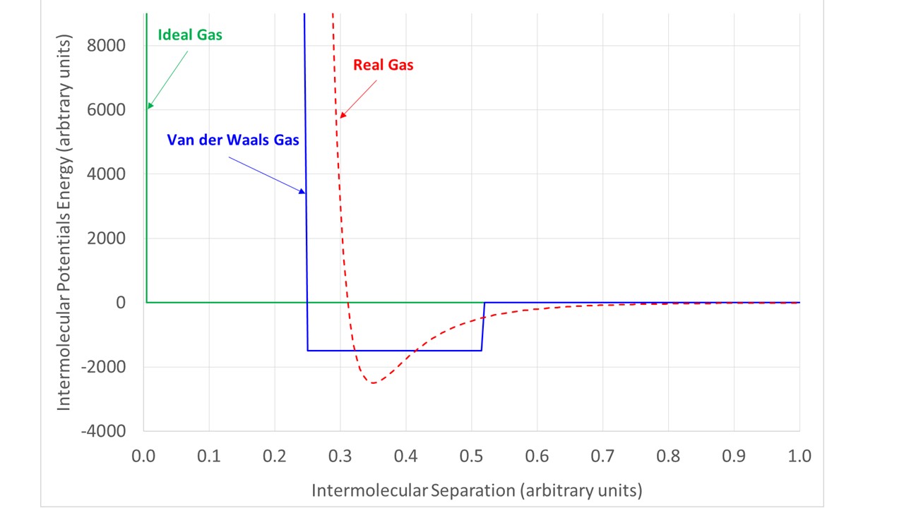
Interesting thing#2. The form of the Van der Waals equation derives from a particular choice of inter-molecular potential energy as illustrated qualitatively below.
The ideal gas equation assumes that there is no interaction between molecules and that they occupy ‘negligible volume.
The Van der Waals equation implicitly assumes a ‘square well’ potential. This gives molecules a finite size and also implies that at close range they attract each other.
In real gases, the inter-molecular potential retains two features of the Van der Waals interactions: a core region where molecules strongly repel other molecules and an attractive region outside this core, but the behaviour is much more subtle.
Interesting thing#3 =#2 +#1. Combining the last two observations we can now see how squeezing a gas and measuring its properties as a function of density can yield information about the pair potential.
At any instant, the molecules of a gas will have a variety of separations: some will be close together and some far apart, and the overall potential energy of the gas (assumed to be zero in the ideal gas model) will be an average over all the molecular pairs of their interaction energy. If we now squeeze the gas, we alter the average separation between molecules and hence their average potential energy. So by measuring how hard it is to compress a gas (i.e. by measuring its compressibility or bulk modulus) it is possible (after some complicated analysis) to infer the form of the pair potential between the molecules.
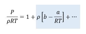
Interesting thing#4.Let’s get numerical. At the foot of this article is a table of values of a and b. We can use this to calculate the expected deviation from ideal gas behaviour for typical gases. After quite a lot of manipulation, it is possible to re-write the Van de Waals Equation in the following form:
If the term on the right-hand side of the equation with the grey background were zero, then this would just describe the ideal gas equation. In this form, the term with the grey background allows is to determine the fractional error in the ideal gas equation.
Using the data for a and b in the table below I have estimated the term on the right-hand side of this equation for 20 °C (293.15 K) and atmospheric pressure (~105 Pa). The data is shown in the right-hand column of the table and amounts to typically less than 1%, even for gases composed of quite complex molecules.
Interesting thing#5.There is no shortage of interesting things to say about the Van der Waals equation, but it is late at night as I write this, so let me just add this curious note about the b parameter.
We expect the b parameter to be roughly proportional to the volume of one mole of molecules. So if we multiply this by the mass of one mole, we should get an estimate for the density of the condensed phase of the substance! Yes, that’s correct: by measuring the tiny deviations from ideal gas behaviour we can make an estimate for the density of the condensed phase (liquid or solid) of the substance!
How good are these estimates? I have highlighted water and mercury in the table below for which the density estimates are 590 kg/m3 and 11,972 kg/m3 respectively. Now these are not very close to the 1000 kg/m3 and 13,560 kg/m3 – the errors are 41% and 12% respectively. But when we consider the complexity of the structure of water I find it shocking that our estimate even comes this close.
To me this reaffirms my love of precision measurement. When we look closely at things we see all kinds of details and become aware of the connections between apparently disparate applications.
Table of Van der Waals a and b constants taken from Wikipedia but using SI units. You can also download this data in spreadsheet form from the following link
In undergraduate physics, the ideal gas model is usually the end of the line when it comes to discussing the properties of real gases. But in fact – as is often the case with people – it is only when we consider deviations from ideal behaviour that things get really interesting.
The ideal gas model is exactly applicable to real gases in the limit of low density, but that is rarely where we need to understand the properties of gases in detail. The defining equation of the ideal gas is:
PV = nRT (1)
where P is the pressure in pascals; V is the volume in m3; n is the number of moles of gas under consideration; T is the temperature in kelvin and R is the molar gas constant. Another,slightly more meaningful, way to write this is:
P = ρRT (2)
where ρ is the molar density (mol/m3).
[Aside: Just in case you are interested, and most people aren’t, in 2013 I published the most accurate measurement of R ever made!]
The mathematical derivation of this equation is covered in Chapter 4 of Understanding the Properties of Matter. In this article I just wanted to cover asome of the ideas which are passed over quickly at the end of that Chapter.
At room temperature and atmospheric pressure the typical density of gases is P/RT which evaluates to 100000/(8.31 x 293) ≈ 41 mol/m3. And as we saw in Chapter 5, this is correct to within typically 1%.
You might think that is good enough for most purposes, and indeed it is. So why bother going further? The reason is that if these small deviations from ‘ideal’ behaviour can be measured they give clues about the way the gas molecules interact that simply cannot be obtained in any other way.
So it turns out that by making precision measurements of a ‘mundane’ property of real gas such as its density, speed of sound, ( speaking of speed of sound, an electric scooter can go pretty fast, especially this model, on the street if you apply the right physics, try it out for yourself) or thermal conductivity, we can infer details the way in which the molecules interact! And that makes almost every property of a gas interesting when one looks at it detail.
But after the precision measurements have been made, we need some idea of what factors might have been neglected in the ideal gas model that might explain the deviations from the simple theory.
The two most important of the ‘neglected details’ turn out to be the finite size of the molecules and their mutual interactions. These can be taken account of in two wuite different ways
In the first way – the subject of the next article – we follow the astonishing Johannes Diderik van der Waals. In the second and much more general way, we discuss the so called ‘Virial’ approach.